
As a follow-up to one of the previous articles that I had created. I wanted to have a backup of this data, and also be able to access it from more than just my computer. My solution to this problem is to put this data in Google Sheets since this allows me to achieve both of my goals. Also, I know that not everyone uses Excel so why not.
While it is not as easy in Excel. It’s still different enough that I decided to put together another blog post documenting the steps.
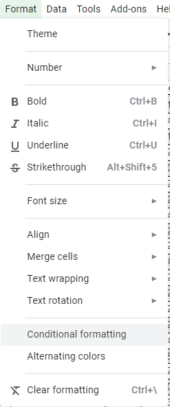
Starting highlight the row, column, or data you want this to be applied on and in the top menu bar click on “Format”, and in the drop-down menu select “Conditional formatting”.
From here a new menu will appear on the right of your screen. Click on ”+ Add another rule” when this section appears choose “Color scale” from the top menu and click on the section noted as “preview”. Now choose a color scale of your liking, for me it is “green to yellow to red”, this is an easy solution for me to know what ones I need to re-evaluate.


 The only issue I have with this color scheme is that the colors are backward. (newest is red oldest is green) This is an easy fix I swapped the colors from the “Min value” and the “Max value”. By doing so I now have the color scheme of my liking and applied to the data I had selected.

 I still don’t have this data being automated yet, but at least I have this in an easier to access format and with some form of backup in case my computer decides to crash and burn.
Hopefully you were able to find this information helpful, Thank you for stopping by.